Frontiers in New-Quality Communication Technology

A fast decoding algorithm for polar codes based on soft output

  • Yiqiao LU 1 ,
  • Yin XU , 1, 3, * ,
  • Hao JU 1 ,
  • Wenxue SUN 1 ,
  • Dongdong WANG 3, 4 ,
  • Dazhi HE 1 ,
  • Yongpeng WU 2 ,
  • Zhiyong CHEN 1 ,
  • Wenjun ZHANG 1, 2
Expand
  • 1. Cooperative Medianet Innovation Center, Shanghai Jiao Tong University, Shanghai 200240, China
  • 2. Department of Electronic Engineering, Shanghai Jiao Tong University, Shanghai 200240, China
  • 3. National Key Laboratory of Advanced Communication Networks, Shijiazhuang 050081, China
  • 4. Academy for Network and Communications of CETC, Shijiazhuang 050081, China

Received date: 2024-11-21

  Online published: 2025-11-07

Copyright

All rights reserved. Unauthorized reproduction is prohibited.

Abstract

Objective: The development of communication systems and increasing demand for low-latency and high-reliability communications has led to a rise in application scenarios requiring soft information interaction for joint iterative decoding to improve system performance. The soft-output successive cancellation list (SO-SCL) decoding algorithm of polar codes can achieve relatively accurate soft information output and decoding with the complexity of traditional successive cancellation list (SCL) decoding by estimating the codebook and posterior probabilities. However, the serial characteristics of SCL decoding result in a high decoding delay of the SO-SCL decoding algorithm, making it difficult to satisfy the 1 Tbps peak throughput requirement of the sixth-generation mobile communication system. To reduce the decoding delay, the existing soft-output fast SCL decoding algorithm (SO -FSCL) realizes fast decoding by identifying four special nodes; however, some nodes still have a high decoding delay. Therefore, a high-performance soft-output decoding algorithm for polar codes with lower decoding delay is required. Methods: In previous studies, special nodes were identified, aiming to achieve fast decoding of different special nodes and combined decoding between nodes. Based on the SO -FSCL decoding algorithm, this study introduces five other special nodes, namely REP-2, REP-3, REP-4, SPC-2, and SPC-3, and proposes a faster soft-output SCL decoding algorithm (FS-SCL). The developed decoding algorithm enables fast decoding of the five new nodes and provides a posterior probability formula for the deleted path. For the REP-2, REP-3, and REP-4 nodes, only 4, 8, and 16 possible decoding paths need to be considered, respectively, and the sum of the probabilities of the deleted paths is calculated. According to the distribution characteristics of the information bits in the nodes, SPC-2 can be simplified to the parallel decoding of two SPC sub-nodes with Ns/2 bits. After combination, the SPC-3 node can be regarded as a repetitive code with a code rate of 1, thereby simplifying the decoding process. Moreover, compared with SCL decoding, which requires flipping all bits, while with the SPC-2 and SPC-3 nodes, only the min{L-1, Ns-2}, min{L-1, Ns-3} bits require flipping during the decoding process, thereby reducing the decoding delay. The time steps required for decoding different nodes are also analyzed herein to evaluate the decoding delay. The five newly added nodes require 3, 4, 5, max{log2Ns+1, min{L, Ns-1}}, and max{log2Ns+3, min{L, Ns-2}} time steps, respectively. Compared with the original SCL decoding algorithm, the node significantly reduces the time steps required for decoding. Results: The simulation results show that by employing the AWGN channel, the proposed FS-SCL decoding algorithm maintains a BER performance similar to that of SO-SCL in different modulation methods, especially under 16QAM. By reducing the proportion of high-code rate nodes, the performance loss is reduced. Compared with the existing SO -FSCL decoding algorithm, the FS-SCL decoding algorithm can further reduce the decoding delay by more than 12.5% (up to 28.7%) and can further reduce the decoding complexity. Moreover, by merging shorter nodes, the FS-SCL decoding algorithm reduces the number of nodes by 42% and achieves a minimum node code length of 8, which is conducive to improving the decoding parallelism. Conclusions: The developed FS-SCL decoding algorithm with lower delay and complexity affords lossless BER performance using different modulation methods. The research results can provide an efficient polar-code decoding scheme for low-latency communication scenarios with soft output, which has important theoretical value and application prospects.

Cite this article

Yiqiao LU , Yin XU , Hao JU , Wenxue SUN , Dongdong WANG , Dazhi HE , Yongpeng WU , Zhiyong CHEN , Wenjun ZHANG . A fast decoding algorithm for polar codes based on soft output[J]. Journal of Tsinghua University(Science and Technology), 2025 , 65(11) : 2032 -2041 . DOI: 10.16511/j.cnki.qhdxxb.2025.27.043

极化码作为一种新型信道编码方式,由土耳其学者Arikan于2008年提出[1],这也是第一个被严格证明能够达到Shannon极限的编码方式。经过广泛研究,极化码在短码长场景下的性能显著优于Turbo码和低密度奇偶校验码(low-density parity-check code,LDPC),成为5G增强移动宽带场景下控制信道的编码方案[2]
针对极化码的解码算法,Arikan[1]提出了基于硬判决的连续消除(successive cancellation,SC)译码算法,利用对数似然比(log likelihood ratio,LLR)和已估计的比特逐个计算信息比特。之后,Arikan[3]进一步将基于软信息的置信传播(belief propagation,BP)算法用于极化码译码,该算法性能优于SC译码但复杂度较高。
在SC译码的基础上,Tal和Vardy[4]提出了连续消除列表(successive cancellation list,SCL)译码算法,通过保留可靠性最高的L条译码路径以降低SC译码中错误传递带来的影响,极大地提高了译码性能。目前,结合循环冗余校验(cyclic redundancy check,CRC)码,CRC辅助的SCL(CRC-aided SCL,CA-SCL)译码[5]是应用范围最广的极化码译码算法。
随着通信领域的发展,多输入多输出(multiple-input multiple-output,MIMO)系统[6]、稀疏码多址(sparse code multiple access,SCMA)[7]、基于极化码的广义码内部迭代[8]等应用场景需要软输入软输出(soft input soft output,SISO)的极化码解码器来实现联合迭代解码。为此,Fayyaz等[9-10]提出了比BP译码复杂度更低的软消除(soft cancellation,SCAN)译码算法。Pillet等[11]和Elkelesh等[12]分别提出了软消除列表译码(soft cancellation list,SCANL)和置信传播列表(belief propagation list,BPL)译码算法,以进一步提升译码性能。
为获得更精确的译码软输出结果,卷积码中常用的BCJR算法[13]被引入极化码进行软输出解码。该算法通过对后验概率进行最优估计来计算极化码的译码软信息,但译码复杂度随码长指数级增长,因此难以实际应用。Pyndiah[14]提出了基于SCL算法的软信息译码方法,通过对后验概率LLR进行估计来降低复杂度,但需要设置饱和阈值以避免无穷值。Yuan等[15]提出SO-SCL译码算法,通过码本概率对Pyndiah近似算法进行了修正,以SCL的译码复杂度实现了接近BCJR算法性能的软输出译码。
由于串行特性,SC和SCL译码存在复杂度高、时延较大等问题。为了降低复杂度和时延,研究者们采用识别特殊节点的方法以实现快速译码。Alamdar-Yazdi等[16]首次提出了码率1(Rate-1)和码率0(Rate-0)节点的快速译码,Sarkis等[17]在此基础上提出了重复码(REP)、单奇偶校验(SPC)节点的简化译码算法。之后,研究者们提出了更多特殊节点以及节点之间的组合[18-19]。Shen等[20]在Yuan等[15]研究的基础上提出软输出的快速SCL(SO-FSCL)译码,将最常见的4种快速译码节应用于SO-SCL译码,能够在几乎不损失性能的条件下实现译码时延显著降低。
本文在Shen等[20]研究的4种节点的基础上,参考Ardakani等[19]的研究划分REP-2、REP-3、REP-4、SPC-2、SPC-3等5种新的节点,并根据节点的特点提出对应的软输出快速译码算法,最终形成包含9种节点的快速译码算法。此外,本文还分析了不同译码算法中节点对应的译码时延并加以比较。

1 基本原理

1.1 极化码

一组二进制极化码可由(N, K)表示,其中N=2n表示码长,K表示信息比特数(亦指传输信息比特的子信道个数)。通过Bhattacharyya参数[1]或Gauss近似法[21]可以对极化子信道的可靠性进行估计,从N个子信道中选出可靠性最高的K个子信道传输信息比特,索引用$ \mathcal{A}$表示,其余传输冻结比特,索引用$ \mathcal{F}$表示。
极化码可以通过待编码比特序列uN={u1, u2, …, uN}与生成矩阵GN=BNFn相乘得到,即
$\boldsymbol{c}^{N}=\boldsymbol{u}^{N} \cdot \boldsymbol{G}_{N}.$
其中BN为位反转矩阵,$ \boldsymbol{F}^{\otimes _n}$表示$ \boldsymbol{F}=\left[\begin{array}{ll}1 & 0 \\ 1 & 1\end{array}\right]$n次Kronecker积,uN也可用u[1, N]表示,本文中设定[1, N]表示{1, 2, …, N}。

1.2 SC、SCL译码算法

SC译码算法通过先前解码结果与LLR来逐步解码每个信息比特,如公式(1)所示。
$\hat{u}_{i}= \begin{cases}0, & i \in \mathcal{F} ; \\ \underset{u_{i} \in\{0, 1\}}{\arg } \max P_{\boldsymbol{Y}^{N}, \boldsymbol{U}^{i-1} \mid U_{i}}\left(\boldsymbol{y}^{N}, \hat{\boldsymbol{u}}^{i-1} \mid u_{i}\right), & i \in \mathcal{A} .\end{cases}$
其中:PYN, Ui-1|Ui$ \left(\boldsymbol{y}^{N}, \hat{\boldsymbol{u}}^{i-1} \mid u_{i}\right)$为给定ui比特下信道接收信号yN和之前译码序列$ \hat{\boldsymbol{u}}^{i-1}$的概率。
SCL译码算法采用多条路径选择的方法来降低部分译码比特出错导致错误传递的影响,其核心原理是设置路径度量(path metric,PM)作为衡量译码路径可靠性的指标,如式(2)所示。
$\mathrm{PM}_{i}^{(l)}=\sum\limits_{k=1}^{i} \ln \left(1+\exp \left(-\left(1-2 \hat{u}_{k}^{(l)}\right) \lambda_{k}^{(l)}\right)\right).$
其中PMi(l)表示第l条路径中第1~i个译码比特的路径度量,$ \hat{u}_{k}^{(l)}$为第l条路径中第k个比特译码结果,对数似然比λk(l)可表示为
$\lambda_{k}^{(l)}=\ln \frac{P_{\boldsymbol{Y}^{N}, \boldsymbol{U}_{[1, k-1]}^{(l)} \mid U_{k}^{(l)}}\left(\boldsymbol{y}^{N}, \hat{\boldsymbol{u}}_{[1, k-1]}^{(l)} \mid 0\right)}{P_{\boldsymbol{Y}^{N}, \boldsymbol{U}_{[1, k-1]}^{(l)} \mid U_{k}^{(l)}}\left(\boldsymbol{y}^{N}, \hat{\boldsymbol{u}}_{[1, k-1]}^{(l)} \mid 1\right)} .$
其中:$ \hat{\boldsymbol{u}}_{[1, k-1]}^{(l)}$表示第l条路径中前(k-1)个比特序列。

1.3 SO-SCL译码算法

SO-SCL译码的核心是引入了码本概率[15],即所有有效译码路径的概率之和,可以理解为满足冻结比特约束的所有可能的译码路径的后验概率之和,如式(3)所示。
$P_{\mathcal{U}}\left(\boldsymbol{y}^{N}\right)=\sum\limits_{\boldsymbol{u}^{N} \in \mathcal{U}} P_{\boldsymbol{U}^{N} \mid \boldsymbol{Y}^{N}}\left(\boldsymbol{u}^{N} \mid \boldsymbol{y}^{N}\right).$
其中:集合$ \mathcal{U}=\left\{\boldsymbol{u}^{N} \in\{0, 1\}^{N}: u_{i}=0, i \in \mathcal{F}\right\}$,后验概率可以通过路径度量PM加以计算:
$P_{\boldsymbol{U}^{i} \mid \boldsymbol{Y}^{N}}\left(\boldsymbol{a}^{i} \mid \boldsymbol{y}^{N}\right)=\exp \left(-\operatorname{PM}\left(\boldsymbol{a}^{i}\right)\right).$
其中:PM(ai)为任意译码路径ai的路径度量。
Yuan等[15]将译码二叉树分为3个部分:已访问的叶节点、无效子树、未访问子树,分别对应于L条译码路径、冻结比特为根节点的子树、译码路径被删除的子树,分别可用集合$ \mathcal{V} $$ \mathcal{J} $$ \mathcal{W} $来表示。因此式(3)中的$ \mathrm{P}_{\mathcal{U}}\left(\boldsymbol{y}^{N}\right)$可以简化为
$\begin{gather*}P_{\mathcal{U}}\left(\boldsymbol{y}^{N}\right) \approx \sum\limits_{\boldsymbol{u}^{N} \in \mathcal{V}} P_{\boldsymbol{U}^{N} \mid \boldsymbol{Y}^{N}}\left(\boldsymbol{u}^{N} \mid \boldsymbol{y}^{N}\right)+ \\\sum\limits_{\boldsymbol{a}^{i} \in \mathcal{W}} 2^{-|\mathcal{F}(i: N)|} P_{\boldsymbol{U}^{i} \mid \boldsymbol{Y}^{N}}\left(\boldsymbol{a}^{i} \mid \boldsymbol{y}^{N}\right).\end{gather*}$
其中:$ \mathcal{F}(i: N)=\{k: k \in \mathcal{F}, i \leqslant k \leqslant N\}, \mid \mathcal{F}(i:N) \mid$为集合中元素的个数。
在进行SCL译码的同时,需要计算每条删除路径对应的概率,最后与译码路径的后验概率相加得到码本概率$ P_{\mathcal{U}}\left(\boldsymbol{y}^{N}\right)$。通过式(6)可以计算每个比特$ \hat{c}_{i}$对应的后验概率对数似然比$ l_{\mathrm{APP}, i}$,其中集合$ \mathcal{C}=\left\{\boldsymbol{c}^{N}: \boldsymbol{c}^{N}=\boldsymbol{u}^{N} \cdot \boldsymbol{F}^{\otimes_{n}}, \boldsymbol{u}^{N} \in \mathcal{U}\right\}$$ P_{\boldsymbol{c}^{N} \mid \boldsymbol{Y}^{N}}\left(\boldsymbol{c}^{N} \mid\right. \left.\boldsymbol{y}^{N}\right)=P_{\boldsymbol{U}^{N} \mid \boldsymbol{Y}^{N}}\left(\boldsymbol{u}^{N} \mid \boldsymbol{y}^{N}\right)$.
$\begin{gather*}l_{\mathrm{APP}, i}=\ln \frac{P_{C_{i} \mid \boldsymbol{Y}^{N}}\left(0 \mid \boldsymbol{y}^{N}\right)}{P_{C_{i} \mid \boldsymbol{Y}^{N}}\left(1 \mid \boldsymbol{y}^{N}\right)}=\ln \frac{\sum\limits_{c_{i}=0, \boldsymbol{c}^{N} \in \mathcal{C}} P_{\boldsymbol{C}^{N} \mid \boldsymbol{Y}^{N}}\left(\boldsymbol{c}^{N} \mid \boldsymbol{y}^{N}\right)}{\sum\limits_{c_{i}=1, \boldsymbol{c}^{N} \in \mathcal{C}} P_{\boldsymbol{C}^{N} \mid \boldsymbol{Y}^{N}}\left(\boldsymbol{c}^{N} \mid \boldsymbol{y}^{N}\right)} \approx \\\ln \frac{\sum\limits_{c_{i}=0, \boldsymbol{c}^{N} \in \mathcal{V}} P_{\boldsymbol{C}^{N} \mid \boldsymbol{Y}^{N}}\left(\boldsymbol{c}^{N} \mid \boldsymbol{y}^{N}\right)+\left[P_{\mathcal{U}}\left(\boldsymbol{y}^{N}\right)-\sum\limits_{\boldsymbol{c}^{N} \in \mathcal{V}} P_{\boldsymbol{C}^{N} \mid \boldsymbol{Y}^{N}}\left(\boldsymbol{c}^{N} \mid \boldsymbol{y}^{N}\right)\right] \cdot P_{C \mid Y}\left(0 \mid y_{i}\right)}{\sum\limits_{c_{i}=1, \boldsymbol{c}^{N} \in \mathcal{V}} P_{\boldsymbol{C}^{N} \mid \boldsymbol{Y}^{N}}\left(\boldsymbol{c}^{N} \mid \boldsymbol{y}^{N}\right)+\left[P_{\mathcal{U}}\left(\boldsymbol{y}^{N}\right)-\sum\limits_{\boldsymbol{c}^{N} \in \mathcal{V}} P_{\boldsymbol{C}^{N} \mid \boldsymbol{Y}^{N}}\left(\boldsymbol{c}^{N} \mid \boldsymbol{y}^{N}\right)\right] \cdot P_{C \mid Y}\left(1 \mid y_{i}\right)}, \quad 1 \leqslant i \leqslant N . \end{gather*}$

2 SO-SCL的快速译码

2.1 现有快速译码算法

Shen等[20]在Yuan等[15]的研究基础上,结合SCL最常用的4种快速译码节点(Rate-0、Rate-1、REP、SPC),实现了SO-SCL的快速译码。假定每个节点$ \mathbb{N}_{i_{\mathrm{s}}}^{j_{\mathrm{s}}}$可由极化子码(Ns, Ks)表示,包含比特的索引可表示为[is, js], js=is+Ns-1,节点中的冻结比特、信息比特索引可由$ \mathcal{F}^{{\rm{s}}}$$ \mathcal{A}^{{\rm{s}}}$表示。该节点的编码比特可通过s[is, js]=u[is, js]Fn得到。译码过程中被删除的路径概率由$ P_{\mathcal{W}}\left(\mathbb{N}_{i_{\mathrm{s}}}^{j_{\mathrm{s}}}\right.$, $ \left.\mathit{\Gamma}\left(\mathbb{N}_{i_{\mathrm{s}}}^{j_{\mathrm{s}}}\right)\right)$表示,其中Γ(·)表示节点对应的类型。
为了简化译码算法,每个节点不再逐个比特译码,而是直接得到译码结果和路径度量。同时,路径度量的计算也与式(4)不同,具体如式(7)所示。
$\mathrm{PM}_{j_{\mathrm{s}}}^{(l)}=\mathrm{PM}_{i_{\mathrm{s}}-1}^{(l)}+\sum\limits_{k=1}^{N_{\mathrm{s}}} \ln \left[1+\exp \left(-\left(1-2 \hat{s}_{k}^{(l)}\right) \alpha_{k}^{(l)}\right)\right].$
其中:$ \hat{s}_{k}^{(l)}$为第l条(1≤lL)路径中当前节点第k个比特的估计码字,αk(l)为当前比特的LLR。得到节点估计码字后,可以通过$ \hat{\boldsymbol{u}}_{\left[i_{\mathrm{s}}, j_{\mathrm{s}}\right]}^{(l)}=\hat{\boldsymbol{s}}_{\left[i_{\mathrm{s}}, j_{\mathrm{s}}\right]}^{(l)} \boldsymbol{F}^{\otimes n}$得到节点对应的译码比特序列。
Rate-0、REP、Rate-1、SPC节点的译码算法如下:
1) Rate-0节点:$ \mathcal{A}^{s}=\emptyset$,所有比特均为冻结比特,故译码比特和编码比特均为0。该节点只有这一种译码结果,因此无需进行路径分裂,故删除路径概率$ P_{\mathcal{W}}(\mathbb{N}_{i_{{\rm{s}}}}^{j_{{\rm{s}}}}$, Rate-0)=0。
2) REP节点:$ \mathcal{A}^{{\rm{s}}}=\left\{N_{{\rm{s}}}\right\}$,只有最后一个比特ujs传递信息比特。因此REP节点只有$ \hat{u}_{j_{{\rm{s}}}}=0$$ \hat{u}_{j_{\mathrm{s}}}=1$这2种译码结果,对应$ \hat{\boldsymbol{s}}_{\left[i_{\mathrm{s}}, j_{\mathrm{s}}\right]}^{(l)}$为全0序列或全1序列,每条路径分裂为2条候选码字,最终在2L条路径中保留PM最小的L条路径,剩余路径被删除并计算概率。
$\begin{gathered}P_{\mathcal{W}}\left(\mathbb{N}_{i_{\mathrm{s}}}^{j_{\mathrm{s}}}, \operatorname{REP}\right)= \\\sum\limits_{\boldsymbol{a}^{j_{\mathrm{s}}} \in \mathcal{W}_{\left[i_{\mathrm{s}}, j_{\mathrm{s}}\right]}^{\mathrm{REP}}} 2^{-\left|\mathcal{F}\left(j_{\mathrm{s}}: N\right)\right|} P_{\boldsymbol{U}^{j_{\mathrm{s}}} \mid \boldsymbol{Y}^{N}}\left(\boldsymbol{a}^{j_{\mathrm{s}}} \mid \boldsymbol{y}^{N}\right) .\end{gathered}$
其中$ \mathcal{W}_{\left[i_{{\rm{s}}}, j_{{\rm{s}}}\right]}^{\mathrm{REP}}$为节点$ \mathbb{N}_{i_{{\rm{s}}}}^{j_{{\rm{s}}}}$中被删除路径的集合。
3) Rate-1节点:$ \mathcal{F}^{{\rm{s}}}=\varnothing$,该节点全部传递信息比特。为降低译码复杂度,采用比特翻转的方法搜索PM最小的L条路径。首先,通过对节点LLR进行硬判决得到第一条最大似然(maximum likelihood,ML)码字,第二条码字则在ML码字的基础上翻转可靠性最小的比特。L条路径分裂为2L条,并保留PM最小的L条路径。接下来,按照可靠性大小排序,对L条路径分别进行不翻转和翻转1个比特的2种操作将会形成2L条路径,保留PM最小的L条路径。重复以上操作,直到翻转比特的次数为min(L-1, Ns)时译码结束。翻转次数的设定将在2.2节中进行解释。删除路径的概率如式(8)所示。
$\begin{align*}& P_{\mathcal{W}}\left(\mathbb{N}_{i_{\mathrm{s}}}^{j_{\mathrm{s}}}, \text { Rate-1 }\right)=2^{-\left|\mathcal{F}\left(j_{\mathrm{s}}: N\right)\right|} . \\& \left(\sum\limits_{\boldsymbol{a}^{i_{\mathrm{s}}-1} \in \mathcal{V}_{i_{\mathrm{s}}-1}^{\text {Node }}} P_{\boldsymbol{U}^{i_{\mathrm{s}}-1} \mid \boldsymbol{Y}^{N}}\left(\boldsymbol{a}^{i_{\mathrm{s}}-1} \mid \boldsymbol{y}^{N}\right)-\right. \\& \left.\sum\limits_{\left.\boldsymbol{a}^{j_{\mathrm{s}}} \in \mathcal{V}_{\left[i_{\mathrm{s}}, j_{\mathrm{s}}\right]}^{\text {Node }}\right]} P_{\boldsymbol{U}^{j_{\mathrm{s}}} \mid \boldsymbol{Y}^{N}}\left(\boldsymbol{a}^{j_{\mathrm{s}}} \mid \boldsymbol{y}^{N}\right)\right) . \end{align*}$
其中$ \mathcal{V}_{\left[i_{{\rm{s}}}, j_{{\rm{s}}}\right]}^{\text {Node }}$$ \mathcal{V}_{i_{{\rm{s}}}-1}^{\text {Node }}$为节点$ \mathbb{N}_{i_{{\rm{s}}}}^{j_{{\rm{s}}}} $$ \mathbb{N}_{1}^{i_{{\rm{s}}}-1}$中已访问的路径集合。
4) SPC节点:$ \mathcal{F}^{{\rm{s}}}=\{1\}$,只有uis传递冻结比特。该比特可视为奇偶校验码,因此SPC节点需要满足所有比特模2和为0的要求。与Rate-1节点类似,首先通过对节点LLR进行硬判决得到ML码字,根据是否满足奇偶校验选择性地翻转可靠性最小的比特作为第一条候选路径。其余操作与Rate-1节点相同,翻转其余比特时,选择性地翻转可靠性最小的比特来满足奇偶校验。翻转比特的次数为min(L-1, Ns-1)。删除路径的概率如下所示,与式(8)类似。
$\begin{gathered}P_{\mathcal{W}}\left(\mathbb{N}_{i_{\mathrm{s}}}^{j_{\mathrm{s}}}, \mathrm{SPC}\right)=2^{-\left|\mathcal{F}\left(j_{\mathrm{s}}: N\right)\right|} \cdot \\\left(\sum\limits_{\boldsymbol{a}^{i_{\mathrm{s}}-1} \in \mathcal{V}_{i_{\mathrm{s}}-1}^{\text {Node }}} P_{\boldsymbol{U}^{i_{\mathrm{s}}-1} \mid \boldsymbol{Y}^{N}}\left(\left[\boldsymbol{a}^{i_{\mathrm{s}}-1}, 0\right] \mid \boldsymbol{y}^{N}\right)-\right. \\\left.\sum\limits_{\left.\boldsymbol{a}^{j_{\mathrm{s}}} \in \mathcal{V}_{\left[i_{\mathrm{s}}\right.}^{\text {Node }} j_{\mathrm{s}}\right]} P_{\boldsymbol{U}^{j_{\mathrm{s}}} \mid \boldsymbol{Y}^{N}}\left(\boldsymbol{a}^{j_{\mathrm{s}}} \mid \boldsymbol{y}^{N}\right)\right) .\end{gathered}$

2.2 本研究提出的译码算法

为了进一步降低译码时延,本研究参考Ardakani等[19]的研究提出了一种更快速的软输出SCL译码算法(FS-SCL),实现包含Rate-1、Rate-0、REP、REP-2、REP-3、REP-4、SPC、SPC-2、SPC-3节点在内的9种节点的快速译码以及软信息的计算。其中Rate-1、Rate-0、REP、SPC节点已在2.1节进行描述,本节不再赘述。
1) REP-2节点
$ \mathcal{A}^{\mathrm{s}}=\left\{N_{\mathrm{s}}-1, N_{\mathrm{s}}\right\}$,只有最后2个比特ujs-1, ujs传递信息比特。该节点的编码比特满足以下规律:
$\boldsymbol{c}_{\left[i_{\mathrm{s}}, j_{\mathrm{s}}\right]}=\left[u_{j_{\mathrm{s}}-1} \oplus u_{j_{\mathrm{s}}}, u_{j_{\mathrm{s}}}, \cdots, u_{j_{\mathrm{s}}-1} \oplus u_{j_{\mathrm{s}}}, u_{j_{\mathrm{s}}}\right].$
即2个信息比特的编码的重复,因此REP-2节点可以看作2个具有Ns/2个比特的REP子树的并行译码,共有$ \left[\hat{u}_{j_{{\rm{s}}}-1}, \hat{u}_{j_{{\rm{s}}}}\right]$为[0, 0]、[0, 1]、[1, 0]、[1, 1]4种译码结果。
由于路径度量满足:
$\ln (1+\exp (a))-\ln (1+\exp (-a))=a .$
其中:a为译码比特为1时的可靠性。即译码比特为1时的PM等于译码比特为0时的PM与对应的LLR之和。因此不同译码结果对应的PM简化如式(9)—(12)所示。
$\mathrm{PM}_{j_{\mathrm{s}}}^{(l)}([0, 0])=\mathrm{PM}_{i_{\mathrm{s}}-1}^{(l)}+\sum\limits_{k=1}^{N_{\mathrm{s}}} \ln \left(1+\exp \left(-\alpha_{k}^{(l)}\right)\right), $
$\mathrm{PM}_{j_{\mathrm{s}}}^{(l)}([0, 1])=\mathrm{PM}_{j_{\mathrm{s}}}^{(l)}([0, 0])+\sigma_{2}, $
$\mathrm{PM}_{j_{\mathrm{s}}}^{(l)}([1, 0])=\mathrm{PM}_{j_{\mathrm{s}}}^{(l)}([0, 0])+\sigma_{1}, $
$\mathrm{PM}_{j_{\mathrm{s}}}^{(l)}([1, 1])=\mathrm{PM}_{j_{\mathrm{s}}}^{(l)}([0, 0])+\sigma_{1}+\sigma_{2} .$
其中$ \sigma_{i}=\sum\limits_{k=0}^{\frac{N_{\mathrm{s}}}{2}-1} \alpha_{2 k+i}^{(l)}, i=1, 2$
实际译码时,每条路径分裂为4条候选码字,最终在4L条路径中保留PM最小的L条路径,剩余路径被删除并计算概率,公式与2.1节中的REP节点类似。
$\begin{gathered}P_{\mathcal{W}}\left(\mathbb{N}_{i_{\mathrm{s}}}^{j_{\mathrm{s}}}, \text { REP- } 2\right)= \\\sum\limits_{\boldsymbol{a}^{j_{\mathrm{s}}} \in \mathcal{W}_{\left[i_{\mathrm{s}}, j_{\mathrm{s}}\right]}^{\mathrm{REPP}-2}} 2^{-\left|\mathcal{F}\left(j_{\mathrm{s}}: \mathrm{N}\right)\right|} P_{\boldsymbol{U}^{j_{\mathrm{s}}} \mid \boldsymbol{Y}^{N}}\left(\boldsymbol{a}^{j_{\mathrm{s}}} \mid \boldsymbol{y}^{N}\right) .\end{gathered}$
2) REP-3节点
$ \mathcal{A}^{{\rm{s}}}=\left\{N_{{\rm{s}}}-2, N_{{\rm{s}}}-1, N_{{\rm{s}}}\right\}$,只有最后3个比特ujs-2, ujs-1, ujs传递信息比特。该节点的编码比特满足以下规律:
$\boldsymbol{c}_{\left[i_{\mathrm{s}}, j_{\mathrm{s}}\right]}=\left[c_{1}, c_{2}, c_{3}, c_{4}, \cdots, c_{1}, c_{2}, c_{3}, c_{4}\right] .$
其中[c1, c2, c3, c4]=[0, ujs-2, ujs-1, ujsF⊗2
REP-3节点可以看作最后4个比特[0, ujs-2, ujs-1, ujs]的编码的重复。该节点共有8种译码结果,信息比特、编码比特集合分别用$ \mathcal{U}_{\left[i_{\mathrm{s}}, j_{\mathrm{s}}\right]}^{\mathrm{REP}-3}$$ \mathcal{C}_{\left[i_{\mathrm{s}}, j_{\mathrm{s}}\right]}^{\mathrm{REP}-3}$表示。
$\begin{gathered}\mathrm{PM}_{j_{\mathrm{s}}}^{(l)}([0,0,0])=\mathrm{PM}_{i_{\mathrm{s}}}^{(l)}+\sum_{k=1}^{N_{\mathrm{s}}} \ln \left(1+\exp \left(-\alpha_{k}^{(l)}\right)\right).\\\mathrm{PM}_{j_{\mathrm{s}}}^{(l)}\left(\boldsymbol{u}_{k}^{\mathrm{REP}-3}\right)=\mathrm{PM}_{j_{\mathrm{s}}}^{(l)}([0,0,0])+\sum_{c_{k}^{\mathrm{REP}-3}[t]=1} \sigma_{t}.\end{gathered}$
其中:$ \sigma_{i}=\sum\limits_{k=0}^{\frac{N_{\mathrm{s}}}{4}-1} \alpha_{4 k+i}^{(l)}, i=\{1, 2, 3, 4\}, \boldsymbol{u}_{k}^{\mathrm{REP}-3}$$ \mathcal{U}_{\left[i_{\mathrm{s}}, j_{\mathrm{s}}\right]}^{\mathrm{REP}-3}$的第k个译码序列,ckREP-3[t]表示编码序列ckREP-3的第t个比特。
实际译码时,每条路径分裂为8条候选码字,最终在8L条路径中保留PM最小的L条路径,删除路径的概率与2.1节中的REP节点一致。
3) REP-4节点
$ \mathcal{A}^{\mathrm{s}}=\left\{N_{\mathrm{s}}-4, ~ N_{\mathrm{s}}-2, ~ N_{\mathrm{s}}-1, ~ N_{\mathrm{s}}\right\}$。Gauss近似法下,(256,128)极化码的极化子信道可靠性如图 1所示,其中信道噪声标准差σ=0.75;局部放大图展示一个REP-4节点的可靠性和信息比特分布,其中可靠性由高至低为ujsujs-1ujs-2ujs-4ujs-3。由于极化码编码和Gauss近似法都是递归式的计算流程,极化子信道的可靠性整体或局部均呈现相同的增长趋势,即任意节点的最后8位比特的可靠性高低排序与小图中展示的相同,因此当一个节点是REP-4时,其中ujs-4, ujs-2, ujs-1, ujs传递信息比特。该节点的编码比特满足如下规律:
$\boldsymbol{c}_{\left[i_{\mathrm{s}}, j_{\mathrm{s}}\right]}=\left[c_{1}, c_{2}, c_{3}, c_{4}, c_{5}, c_{6}, c_{7}, c_{8}, \cdots\right] .$
图 1 (256,128)极化码的极化子信道可靠性
其中[c1, c2, c3, c4, c5, c6, c7, c8]=[0, 0, 0, ujs-4, 0, ujs-2, ujs-1, ujsF⊗3.
该节点共有16种译码结果,信息比特、编码比特集合分别用$ \mathcal{U}_{\left[i_{\mathrm{s}}, j_{\mathrm{s}}\right]}^{\mathrm{REP}-4} $$ \mathcal{C}_{\left[i_{\mathrm{s}}, j_{\mathrm{s}}\right]}^{\mathrm{REP}-4}$表示。
$\begin{gathered}\mathrm{PM}_{j_{\mathrm{s}}}^{(l)}([0, 0, 0, 0])= \\\mathrm{PM}_{i_{\mathrm{s}}-1}^{(l)}+\sum\limits_{k=1}^{N_{\mathrm{s}}} \ln \left(1+\exp \left(-\alpha_{k}^{(l)}\right)\right), \\\mathrm{PM}_{j_{\mathrm{s}}}^{(l)}\left(\boldsymbol{u}_{k}^{\mathrm{REP}-4}\right)=\mathrm{PM}_{j_{\mathrm{s}}}^{(l)}([0, 0, 0, 0])+\sum\limits_{c_{k}^{\mathrm{REP}-4}[t]=1} \sigma_{t} .\end{gathered}$
其中:$ \sigma_i=\sum\limits_{k=0}^{\frac{N_{\mathrm{s}}}{8}-1} \alpha_{8 k+i}^{(l)}, i=\{1, 2, 3, \cdots, 8\}$
REP-4节点译码过程与2.1节中的REP节点类似。
4) SPC-2节点
$ \mathcal{F}^{\mathrm{s}}=\{1, 2\}$,只有前2个比特{u1, u2}传递冻结比特,可看作2个奇偶校验比特。根据极化码的编码特性,可以计算出对应的校验函数。该节点的编码比特满足以下规律:
$p[1]: \oplus c=0, \quad c \in \boldsymbol{c}_{\left[i_{\mathrm{s}}, j_{\mathrm{s}}\right]} ;$
$p[2]: \oplus c=0, \quad c \in \boldsymbol{c}_{\left[i_{\mathrm{s}}, j_{\mathrm{s}}\right]}^{e} ;$
$p[1]+p[2]: \oplus c=0, \quad c \in \boldsymbol{c}_{\left[i_{\mathrm{s}}, j_{\mathrm{s}}\right]}^{o} .$
其中:⊕表示模2和,c[is, js]e={ci, i∈[is, js], i mod 2=0},c[is, js]o={ci, i∈[is, js], i mod 2=1},分别对应序号为偶数、奇数的编码比特集合。
由式(14)和(15)可知,SPC-2节点的2个校验函数涉及的比特没有交集,因此译码时可简化为2个具有Ns/2个比特的SPC子节点的并行译码。
实际译码时,首先对节点比特进行硬判决得到ML码字$ \hat{c}_{\left[i_{\mathrm{s}}, j_{\mathrm{s}}\right]}$,分别计算2个子节点的模2和mo(l), me(l),并找到LLR绝对值最小的比特索引ol, el。若子节点不满足奇偶校验,则翻转可靠性最小的比特,即$ \hat{c}_{o_{l}}=\hat{c}_{o_{l}} \oplus m_{o}^{(l)}, \hat{c}_{e_{l}}=\hat{c}_{e_{l}} \oplus m_{e}^{(l)}$
$\begin{gathered}\mathrm{PM}_{\mathrm{ML}}^{(l)}=\mathrm{PM}_{i_{\mathrm{s}}-1}^{(l)}+\sum\limits_{k=1}^{N_{\mathrm{s}}} \ln \left(1+\exp \left(-\alpha_{k}^{(l)}\right)\right)+ \\m_{o}^{(l)}\left|\alpha_{o_{l}}^{(l)}\right|+m_{e}^{(l)}\left|\alpha_{e_{l}}^{(l)}\right|.\end{gathered}$
然后对节点除$ \hat{c}_{o_{l}}, \hat{c}_{e_{l}}$外的编码比特的可靠性|α[is, js](l)|进行排序,得到索引序列γ。Ardakani等[19]的研究中Theorem 1证明了包含ML码字在内最多只需要翻转min(L, Ns-1)个比特。当i>min(L-1, Ns-2)时,$ \hat{\boldsymbol{c}}_{\gamma_{i}}$无需翻转,只需要保留硬判决结果。因为翻转后的路径PM一定不包含在PM最小的L条路径中,故可简化这部分译码过程。
当1≤i≤min(L-1, Ns-2)时,每条路径分裂为不额外翻转比特和翻转γi比特2种情况,根据是否满足奇偶校验选择性地翻转$ \hat{c}_{o_{l}}, \hat{c}_{e_{l}}$。PM计算方法如式(16)所示,同时更新mo(l)me(l)。此时,共形成2L条候选路径,保留其中PM最小的L条。
$\mathrm{PM}_{\gamma_{i}}^{(l)}=\left\{\begin{array}{l}\mathrm{PM}_{\gamma_{i-1}}^{(l)}, \\\mathrm{PM}_{\gamma_{i-1}}^{(l)}+\left|\alpha_{\gamma_{i}}^{(l)}\right|+\beta_{\gamma_{i}}^{(l)} .\end{array}\right.$
其中PMγ0(l)=PMML(l)。若γi为奇数则βγi(l)=(1-2mo(l))|αol(l)|,反之同理。
删除路径的概率与SPC类似,见式(17)。此时,需要通过fg运算计算第1、2个译码比特$ \hat{\boldsymbol{u}}_{[1, 2]}$对应的LLR,并计算路径度量。
$\begin{gather*}P_{\mathcal{W}}\left(\mathbb{N}_{i_{\mathrm{s}}}^{j_{\mathrm{s}}}, \operatorname{SPC}-2\right)=2^{-\left|\mathcal{F}\left(j_{\mathrm{s}}: N\right)\right|} \cdot \\\left(\sum\limits_{\boldsymbol{a}^{i_{\mathrm{s}}-1} \in \mathcal{V}_{i_{\mathrm{s}}-1}^{\text {Node }}} P_{\boldsymbol{U}^{i_{\mathrm{s}}-1} \mid \boldsymbol{Y}^{N}}\left(\left[\boldsymbol{a}^{i_{\mathrm{s}}-1}, 0, 0\right] \mid \boldsymbol{y}^{N}\right)-\right. \\\left.\sum\limits_{\left.\boldsymbol{a}^{j_{\mathrm{s}}} \in \mathcal{V}_{\left[i_{\mathrm{s}}, j_{\mathrm{s}}\right]}^{\text {Node }}\right]} P_{\boldsymbol{U}^{j_{\mathrm{s}}} \mid \boldsymbol{Y}^{N}}\left(\boldsymbol{a}^{j_{\mathrm{s}}} \mid \boldsymbol{y}^{N}\right)\right) . \end{gather*}$
5) SPC-3节点
$ \mathcal{F}^{\mathrm{s}}=\{1, 2, 3\}$,只有前3个比特u1, u2, u3传递冻结比特,对应3个校验函数。将编码比特按照模4的余数分为4组:c[is, js]i=$ \left\{\hat{c}_{k}, k \in\left[i_{\mathrm{s}}, j_{\mathrm{s}}\right]\right.$, $ k \ {\rm{mod}}\ 4=i\}, i=\{0, 1, 2, 3\}$
$p[1]: \oplus c=0, \quad c \in \boldsymbol{c}_{\left[i_{\mathrm{s}}, j_{\mathrm{s}}\right]} . $
$p[2]: \oplus c=0, \quad c \in \boldsymbol{c}_{\left[i_{\mathrm{s}}, j_{\mathrm{s}}\right]}^{2} \cup \boldsymbol{c}_{\left[i_{\mathrm{s}}, j_{\mathrm{s}}\right]}^{0};$
$p[3]: \oplus c=0, \quad c \in \boldsymbol{c}_{\left[i_{\mathrm{s}}, j_{\mathrm{s}}\right]}^{3} \cup \boldsymbol{c}_{\left[i_{\mathrm{s}}, j_{\mathrm{s}}\right]}^{0};$
$p[2]+p[3]: \oplus c=0, \quad c \in \boldsymbol{c}_{\left[i_{\mathrm{s}}, j_{\mathrm{s}}\right]}^{2} \cup \boldsymbol{c}_{\left[i_{\mathrm{s}}, j_{\mathrm{s}}\right]}^{3};$
$\begin{gather*}p[1]+p[2]+p[3]: \oplus c=0, \\c \in \boldsymbol{c}_{\left[i_{\mathrm{s}}, j_{\mathrm{s}}\right]}^{1} \cup \boldsymbol{c}_{\left[i_{\mathrm{s}}, j_{\mathrm{s}}\right]}^{0} . \end{gather*}$
由式(20)—(22)可得
$\begin{gathered}c_{0} \oplus c_{1}=c_{1} \oplus c_{2}=c_{2} \oplus c_{3}=c_{3} \oplus c_{0}. \\c_{0}=c_{1}=c_{2}=c_{3}=0 \text { or } 1.\end{gathered}$
其中$ c_{i}=\oplus c, c \in \boldsymbol{c}_{\left[i_{\mathrm{s}}, j_{\mathrm{s}}\right]}^{i}$
因此{c0, c1, c2, c3}可以看作码率为1的重复码。实际译码时,既需要满足每组子节点的模2和为0或1,又要满足c0, c1, c2, c3有相同值。
与SPC-2节点类似,SPC-3节点需要获得4个子节点的模2和mt(l)t={0, 1, 2, 3}, 以及对应的LLR绝对值最小的比特索引tl。若子节点不满足奇偶校验,那么翻转可靠性最小的比特,即$ \hat{c}_{t_{l}}= \hat{c}_{t_{l}} \oplus m_{t}{ }^{(l)}$
然后对节点除tl, t={0, 1, 2, 3}外的编码比特的可靠性|α[is, js](l)|进行排序,得到索引序列γ。与SPC-2节点同理,SPC-3节点最多只需要翻转min(L, Ns-2)个比特。
当1≤i≤min(L-1, Ns-3)时,译码过程与2.2节中的SPC-2节点一致。
删除路径的概率与SPC类似,见式(23)。此时,需要通过fg运算计算第1~3个译码比特$ \hat{\boldsymbol{u}}_{[1, 3]}$对应的LLR,并计算路径度量。
$\begin{gather*}P_{\mathcal{W}}\left(\mathbb{N}_{i_{\mathrm{s}}}^{j_{\mathrm{s}}}, \mathrm{SPC}-3\right)=2^{-\left|\mathcal{F}\left(j_{\mathrm{s}}: N\right)\right|} \\\left(\sum\limits_{\boldsymbol{a}^{i_{\mathrm{s}}-1} \in \mathcal{V}_{i_{\mathrm{s}}-1}^{\text {Node }}} P_{\boldsymbol{U}^{i_{\mathrm{s}}-1} \mid \boldsymbol{Y}^{N}}\left(\left[\boldsymbol{a}^{i_{\mathrm{s}}-1}, 0, 0, 0\right] \mid \boldsymbol{y}^{N}\right)-\right. \\\left.\sum\limits_{\left.\boldsymbol{a}^{j_{\mathrm{s}}} \in \mathcal{V}_{\left[i_{\mathrm{s}}, j_{\mathrm{s}}\right.}^{\text {Node }} \right]} P_{\boldsymbol{U}^{j_{\mathrm{s}}} \mid \boldsymbol{Y}^{N}}\left(\boldsymbol{a}^{j_{\mathrm{s}}} \mid \boldsymbol{y}^{N}\right)\right).\end{gather*}$

2.3 译码时延分析

译码时延可以通过解码特定节点所需的时间步长来评估。本研究参考Hashemi等[18]、Ardakani等[19]、Condo[22]等研究中的假设如下:
1) 假设并行执行的操作没有资源限制,也就是说任何并行运算都可以在一个时间步长内完成;
2) 实数的基本操作(fg运算)需要一个时间步长;
3) 硬判决、比特操作和符号判断可以瞬间进行;
4) 获取SPC节点的ML码字需要一个时间步长;
5) 路径分裂、PM排序和最可能路径的选择需要一个时间步长。
根据以上假设,可以求出不同类型节点所需的时间步长,如表 1所示。其中“—”表示对应译码算法中没有该类节点。
表 1 节点长度为Ns、列表大小为时不同节点所需的时间步长
节点类型 时间步长
SO-SCL[15] SO-FSCL[20] FS-SCL(本研究提出)
Rate-0 2Ns-2 1 1
Rate-1 3Ns-2 min{L, Ns+1} min{L, Ns+1}
REP 2Ns-1 2 2
REP-2 2Ns 3
REP-3 2Ns+1 4
REP-4 2Ns+2 5
SPC 3Ns-3 max{log2Ns, min{L, Ns}} max{log2Ns, min{L, Ns}}
SPC-2 3Ns-4 max{log2Ns+1, min{L, Ns-1}}
SPC-3 3Ns-5 max{log2Ns+3, min{L, Ns-2}}
对于常规的SO-SCL译码算法,所有节点均逐比特译码。一个(N, K)极化码需要(2N+K-2)个时间步长生成硬判决结果[18],因此该译码算法每个节点所需的时间步长如表 1所示。
对于快速译码的SO-FSCL、FS-SCL译码算法,不同类型的节点译码时间步长分析如下:
1) Rate-0节点无需路径分裂和排序选择,只包含PM计算所需的1个时间步长。
2) REP、REP-2、REP-3、REP-4节点分别需要进行1、2、3、4次路径分裂以及1次路径排序与选择,故译码时分别需要2、3、4、5个时间步长。
3) Rate-1节点需要1个时间步长来获取硬判决结果和PM计算,min{L-1, Ns}个时间步长进行路径分裂、选择和PM更新,因此译码共需要min{L, Ns+1}个时间步长。
4) 与Rate-1节点相类似,SPC节点的译码也需要1+min{L-1, Ns-1}个时间步长。但由于SPC节点的删除路径概率需要计算译码比特$ \hat{u}_{1}$对应的LLR,因此还需要进行log2Nsfg操作。以上2个操作互不干扰可以并行运算,因此最终译码时需要max{log2Ns, min{L, Ns}}个时间步长。同理,SPC-2节点需要min{L, Ns-1}、(log2Ns+1)个时间步长进行SCL解码和LLR运算。多出的1次LLR运算是因为还需要1次g运算计算译码比特$ {\hat u_2}$的LLR。因此最终需要$ \max \left\{\log _{2} N_{\mathrm{s}}+1, \min \left\{L, N_{\mathrm{s}}-1\right\}\right\}$个时间步长。SPC-3节点额外需要各1次fg运算计算译码比特$ \hat{u}_{3}$的LLR,最终需要max{log2Ns+3, min{L, Ns-2}}个时间步长。

3 实验结果与分析

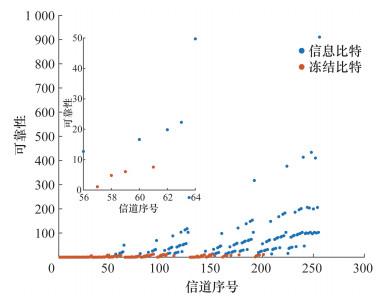
本章将从误比特率(bit error rate, BER)、译码时延、译码复杂度3个方面评估FS-SCL译码算法的性能。仿真实验中,本研究采用Gauss近似方法[21]构造(N, K)极化码,其中冻结比特传输0,并在加性Gauss白噪声(additive white Gaussian noise,AWGN)信道中传输。

3.1 译码误比特率

对比未采用快速译码的SO-SCL译码算法[15]、现有的软输出快速译码算法SO-FSCL[20]和本研究提出的FS-SCL译码算法在不同信噪比(signal noise ratio,SNR)、不同调制方式(BPSK、QPSK、16QAM)下的BER性能,结果如图 2所示,其中列表数量L=2。由图可知,3种不同调制方法下,FS-SCL与未采用快速译码的SO-SCL译码算法相比几乎没有性能损失。其中包含4种快速译码节点的SO-FSCL译码算法在BPSK、QPSK调制下性能几乎无损,但在16-QAM下有一定性能差异。原因可能是SO-FSCL中有较多码率较高的Rate-1、SPC节点,这些节点在高SNR下较为敏感,导致最终的性能损失较为明显。快速译码算法SO-FSCL和FS-SCL不同节点的码长和数量分布以及节点占比如表 2所示,由表可知,FS-SCL通过增加5类新节点,大大减小了原有4种节点的比例。因此本研究提出的FS-SCL译码算法能够实现几乎无损的译码性能。
图 2 不同调制方法下(512,256)极化码(L=2)BER性能曲线
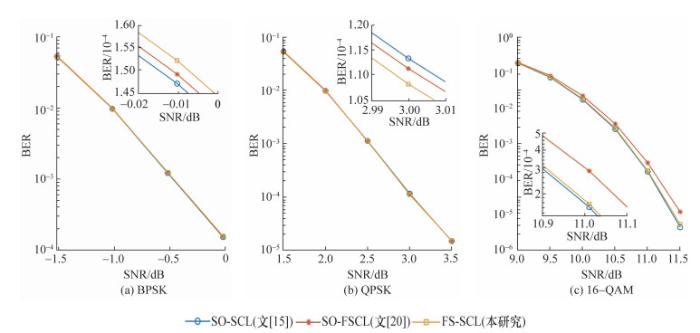
表 2 (512,256)极化码下不同快速译码算法的节点码长和数量
节点类型 SO-FSCL[20] FS-SCL(本研究)
节点码长 节点总数(占比/%) 节点码长 节点总数(占比/%)
2 4 8 16 32 64 8 16 32 64
Rate-0 4 2 3 1 0 1 11(22) 0 0 0 1 1(3.4)
Rate-1 4 3 3 1 0 0 11(22) 2 1 0 0 3(10.3)
REP 0 8 3 1 2 0 14(28) 3 1 2 0 6(20.7)
REP-2 1 1 0 0 2(6.9)
REP-3 0 0 0 0 0(0)
REP-4 5 1 1 0 7(24.1)
SPC 0 7 3 1 2 1 14(28) 3 1 2 1 7(24.1)
SPC-2 1 1 0 0 2(6.9)
SPC-3 1 0 0 0 1(3.4)

3.2 译码时延

3种译码算法在不同码长、码率和列表大小L(即L条译码路径)下的译码延时即时间步长如表 3所示。由表可知,在相同的码长、码率、列表大小条件下,与SO-FSCL相比,FS-SCL减少了12.5%以上的时间步长,最多可减少28.7%,进一步降低了软输出译码过程中的译码时延。对比列表数量L=2和L=4时的时间步长,可以发现:随着L的增大,快速译码所需的时间步长增加。同时,随着L的增加,FS-SCL译码算法相比SO-FSCL时间步长数的减少百分比变大,说明FS-SCL译码算法降低译码时延的幅度大于列表数量增加导致时延增长的幅度。
表 3 不同列表大小下不同节点所需的时间步长
(N, K) L SO-SCL[15] SO-FSCL[20] FS-SCL(本研究) 降低百分比/%
(128,96) 2 350 56 49 12.5
4 69 57 17.4
(256,128) 2 638 112 98 12.5
4 131 105 19.8
(512,256) 2 1 278 202 160 20.8
4 237 169 28.7
(1024,512) 2 2 558 345 281 18.6
4 403 295 26.8

注:“降低百分比”表示本研究提出的FS-SCL译码算法相比SO-FSCL译码算法[20]时间步长的降低百分比。

结合表 2中各快速译码节点的数量和码长可知,SO-FSCL中节点总数为50,其中码长为2或4的节点占比为56%;而FS-SCL中节点总数为29,相比SO-FSCL显著减少,节点的最小码长为8,同时原有的4种节点比例均降低。说明FS-SCL通过增加节点类型能够将部分较短节点合并,从而减少节点个数,增加节点的码长,进一步减少了译码时延,有助于提高译码并行度。

3.3 译码复杂度

为进一步评估译码算法的复杂度,表 4统计了(512,256)极化码在译码过程中所需的f/g运算数量、二叉树节点和边的数量。其中f/g运算为极化码解码的主要运算,公式较为复杂;而极化码译码需要遍历二叉树的节点和边,这些操作也会影响译码的复杂度。由表可知:相比未采用快速译码的SO-SCL,快速译码算法SO-FSCL和FS-SCL的复杂度各指标均大幅度减少,说明采用快速译码能显著降低译码复杂度。与现有的SO-FSCL相比,FS-SCL进一步减少了节点和边的数量,同时f/g运算数量也有所减少,故说明FS-SCL译码算法相比SO-FSCL译码算法能够进一步降低复杂度。
表 4 (512,256)极化码不同译码算法复杂度指标统计
数量 L SO-SCL[15] SO-FSCL[20] FS-SCL(本研究) 降低百分比/%
f/g 2 8 128 4 794 4 434 7.5
4 14 944 8 920 8 144 8.7
节点 2 512 50 29 42.0
4
2 1 851 287 201 30.0
4 3 445 545 381 30.1

注:“降低百分比”表示FS-SCL译码算法的复杂度指标相比SO-FSCL译码算法[20]的降低百分比。

4 结论

本文提出了FS-SCL译码算法,在现有的Rate-0、Rate-1、REP、SPC节点基础上,划分REP-2、REP-3、REP-4、SPC-2、SPC-3等5种新的节点,最终形成共9种节点的快速译码方法。仿真结果表明,所提出的FS-SCL译码算法在不同调制方法中均保持与SO-SCL相近的BER性能,尤其在16QAM下通过减少高码率节点占比,性能损失更小。与现有的SO-FSCL译码算法相比,FS-SCL译码算法进一步降低译码时延12.5%以上,最高达到28.7%,进一步减少译码复杂度;同时通过合并较短节点,FS-SCL译码算法减少了42%的节点个数,实现节点最小码长为8,有利于提高译码并行度。因此,本研究可为低时延的软输出通信场景提供高效的极化码译码方案。
1
ARIKAN E . Channel polarization: A method for constructing capacity-achieving codes for symmetric binary-input memoryless channels[J]. IEEE Transactions on Information Theory, 2009, 55 (7): 3051- 3073.

DOI

2
HUI D , SANDBERG S , BLANKENSHIP Y , et al. Channel coding in 5G new radio: A tutorial overview and performance comparison with 4G LTE[J]. IEEE Vehicular Technology Magazine, 2018, 13 (4): 60- 69.

DOI

3
ARIKAN E . A performance comparison of polar codes and Reed-Muller codes[J]. IEEE Communications Letters, 2008, 12 (6): 447- 449.

DOI

4
TAL I , VARDY A . List decoding of polar codes[J]. IEEE Transactions on Information Theory, 2015, 61 (5): 2213- 2226.

DOI

5
NIU K , CHEN K . CRC-aided decoding of polar codes[J]. IEEE Communications Letters, 2012, 16 (10): 1668- 1671.

DOI

6
DAI J C , NIU K , LIN J R . Polar-coded MIMO systems[J]. IEEE Transactions on Vehicular Technology, 2018, 67 (7): 6170- 6184.

DOI

7
PAN Z P , LI E B , ZHANG L , et al. Design and optimization of joint iterative detection and decoding receiver for uplink polar coded SCMA system[J]. IEEE Access, 2018, 6, 52014- 52026.

DOI

8
SHEN L , WU Y P , XU Y , et al. GLDPC-PC codes: Channel coding toward 6G communications[J]. IEEE Communications Magazine, 2025, 1- 7.

9
FAYYAZ U U , BARRY J R . Low-complexity soft-output decoding of polar codes[J]. IEEE Journal on Selected Areas in Communications, 2014, 32 (5): 958- 966.

DOI

10
FAYYAZ U U, BARRY J R. A low-complexity soft-output decoder for polar codes[C]//2013 IEEE Global Communications Conference (GLOBECOM). Atlanta, USA: IEEE, 2013: 2692-2697.

11
PILLET C, CONDO C, BIOGLIO V. SCAN list decoding of polar codes[C]//ICC 2020-2020 IEEE International Conference on Communications. Dublin, Ireland: IEEE, 2020: 1-6.

12
ELKELESH A , EBADA M , CAMMERER S , et al. Belief propagation list decoding of polar codes[J]. IEEE Communications Letters, 2018, 22 (8): 1536- 1539.

DOI

13
BAHL L , COCKE J , JELINEK F , et al. Optimal decoding of linear codes for minimizing symbol error rate (Corresp.)[J]. IEEE Transactions on Information Theory, 1974, 20 (2): 284- 287.

14
PYNDIAH R M . Near-optimum decoding of product codes: Block turbo codes[J]. IEEE Transactions on Communications, 1998, 46 (8): 1003- 1010.

DOI

15
YUAN P H, DUFFY K R, MÉDARD M. Near-optimal generalized decoding of polar-like codes[C]//2024 IEEE International Symposium on Information Theory (ISIT). Athens, Greece: IEEE, 2024: 2939-2944.

16
ALAMDAR-YAZDI A , KSCHISCHANG F R . A simplified successive-cancellation decoder for polar codes[J]. IEEE Communications Letters, 2011, 15 (12): 1378- 1380.

DOI

17
SARKIS G , GIARD P , VARDY A , et al. Fast polar decoders: Algorithm and implementation[J]. IEEE Journal on Selected Areas in Communications, 2014, 32 (5): 946- 957.

DOI

18
HASHEMI S A , CONDO C , GROSS W J . Fast and flexible successive-cancellation list decoders for polar codes[J]. IEEE Transactions on Signal Processing, 2017, 65 (21): 5756- 5769.

DOI

19
ARDAKANI M H , HANIF M , ARDAKANI M , et al. Fast successive-cancellation-based decoders of polar codes[J]. IEEE Transactions on Communications, 2019, 67 (7): 4562- 4574.

DOI

20
SHEN L, WU Y P, XU Y, et al. Soft-output fast successive-cancellation list decoder for polar codes[C]//2025 IEEE Wireless Communications and Networking Conference (WCNC). Milan, Italy: IEEE, 2025: 1-6.

21
TRIFONOV P . Efficient design and decoding of polar codes[J]. IEEE Transactions on Communications, 2012, 60 (11): 3221- 3227.

DOI

22
CONDO C, BIOGLIO V, LAND I. Generalized fast decoding of polar codes[C]//2018 IEEE Global Communications Conference (GLOBECOM). Abu Dhabi, United Arab Emirates: IEEE, 2018: 1-6.

Outlines

/